線形回帰

Section 02: Basic Knowledge of Deep Learning の Lecture 06: The Transformer Model にて紹介した線形回帰の散布図の描画方法を示します。

疑似データの準備

以下のようにして疑似データを説明変数 \(x\) と被説明変数 \(y\) として準備します。

import numpy as np

N = 30 # サンプル数

x = np.linspace(1, 10, N)
y = x * 5 + np.random.randn(N) * 5

x = x.reshape([-1, 1])
y = y.reshape([-1, 1])

sklearn による線形回帰

sklearn の LinearRegression を使用して \(x\) から \(y\) を予測するように学習させます。

from sklearn.linear_model import LinearRegression

# 線形回帰モデルの準備
clf = LinearRegression()
# x から y を予測できるようにモデルを学習
clf.fit(x, y)

# 学習させたモデルで x に対して予測を実施
y_hat = clf.predict(x)

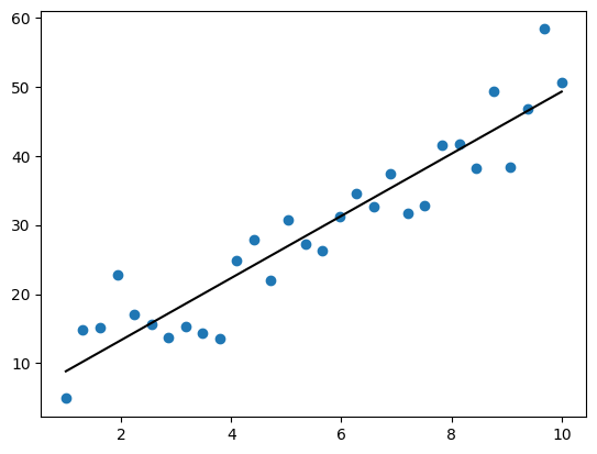
散布図の描画

説明変数 \(x\) 、被説明変数 \(y\) 、そして予測値 \(\hat{y}\) をそれぞれ以下のようにして描画します。

import matplotlib.pyplot as plt

fig, ax = plt.subplots()

ax.scatter(x, y)
ax.plot(x, y_hat, c="black")

[<matplotlib.lines.Line2D at 0x7ef53cc1f190>]