多次元正規分布の描画#
Section 03: Basics of Diffusion Model の Lecture 08: Score-based Generative Model にて使用した2次元正規分布のプロット方法を紹介します。
import numpy as np

#関数に投入するデータを作成
x = y = np.arange(-20, 20, 0.5)
X, Y = np.meshgrid(x, y)

z = np.c_[X.ravel(), Y.ravel()]

#二次元正規分布の確率密度を返す関数
def gaussian(x):
    #分散共分散行列の行列式
    det = np.linalg.det(sigma)
    print(det)
    #分散共分散行列の逆行列
    inv = np.linalg.inv(sigma)
    n = x.ndim
    print(inv)
    return np.exp(-np.diag((x - mu)@inv@(x - mu).T)/2.0) / (np.sqrt((2 * np.pi) ** n * det))
#2変数の平均値を指定
mu = np.array([3,1])
#2変数の分散共分散行列を指定
sigma = np.array([[20,10],[10,20]])
import matplotlib.pyplot as plt
from mpl_toolkits.mplot3d import axes3d
from matplotlib import cm
Z = gaussian(z)
shape = X.shape
Z = Z.reshape(shape)
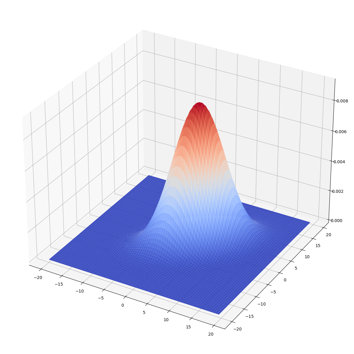
#二次元正規分布をplot
fig = plt.figure(figsize = (15, 15))
ax = fig.add_subplot(111, projection='3d')
ax.plot_surface(X, Y, Z, rstride=1, cstride=1, cmap=cm.coolwarm)
299.99999999999994
[[ 0.06666667 -0.03333333]
 [-0.03333333  0.06666667]]
<mpl_toolkits.mplot3d.art3d.Poly3DCollection at 0x7cada4276650>
参考#
Pythonで学ぶ統計学(5): 同時確率分布 - 投資のためのデータサイエンス https://datapowernow.hatenablog.com/entry/2020/02/23/134631